Biometrics and Statistical Analysis of Data
What Is Biometrics?
In this lab exercise, you will learn more about using metric
system measurements for height and weight, how to read lab equipment and
interpolate digits, and how to calculate averages and standard deviations to
analyze data. Also, in this lab, humans (Homo sapiens) will be used as
an example to illustrate Darwins concept of intraspecific variation.
In biology, as in other sciences, gathering numerical data to
test ones hypothesis and subsequently performing a statistical analysis on
those data are of utmost importance when interpreting the data and drawing
any conclusions from them. Due to a variety of factors, despite the most
careful observations, there will always be some variation in the data
collected, hence the necessity for a statistical analysis of those data.
Biometrics is the application of statistical methodology to analyze
biological data.
Interpolation of Data
In collecting data, it is important to know how to correctly
read the equipment being used. This frequently involves interpolation
to obtain the last digit of the data. Interpolation is reading between the
lines for example, if youre looking at a clock that only has 5-min.
markings on it and you read a time of 8:53, you are interpolating the 3 by
estimating how far between the 0 and the 5 the minute hand of the clock
is. Similarly, when reading the scale on a piece of scientific apparatus,
it is also necessary to interpolate, to read between the lines. For example,
in the illustration, above, if the numbered divisions represent grams, then
the marked divisions in between represent tenths of a gram. This scale must,
then, be read to the one-hundredths of a gram by envisioning ten divisions
in the white space in between the tenth-gram markings.
Also, in biology, as in other sciences, the metric system is used.
Thus, we measure an organisms weight in grams or kilograms and its length
or height in centimeters or meters.
Statistical Analysis
To evaluate these numbers, it is necessary to employ several
statistical concepts. The mean or average
(X)
of a set of data is a measure of central tendency of a group of numbers,
such that the total of the deviations of the numbers above the mean is equal
to the total of the deviations of the numbers below the mean. For example,
for the numbers 1, 3, 5, 7, and 9, the mean is 5, so the deviations of each
of the numbers from that mean are 4, 2, 0, 2, and 4, respectively. Note
that the absolute values of |2 + 4| and |(4) + (2)| are equal. Further,
note that the sum of the deviations around a mean should always be 0. The
mean is the total of the values divided by the number of data points. This
is expressed mathematically as:
X = (ΣXi)/N.
Σ means sum, Xi means all the
individual values, and N means the number
of items. The closer the mean of a group of numbers is to the true value,
the more accurate that mean and group of numbers are.
Another concept that is sometimes used is that of the
median, which is the data point above and below which one-half of the
data points lie. That means that if there is an odd number of data points,
the median is the number thats in the middle of the list, just by counting
in from both ends. If there is an even number of data points, the median is
the average of the middle two. For example, for the numbers 2, 6, 7, 14, and
56, the median is 7. For the numbers 2, 6, 7, 9, 14, and 56, the median is
(7 + 9)/2 = 8.
The mean is preferred over the median as a measure of central
tendency in a group of data, but there might be some situations where the
median would be a better indicator. If a distribution is symmetrical, the
mean and median should be about the same, but if a distribution is skewed,
then the median might be a better measure to use than mean. For example, if
a statistician was looking at family income in an area where four families
had incomes of under $20,000 while one family had an income of over
$1,000,000, then median would be a better indicator of typical family
income in that community. The median is less sensitive to extremes in the
data than the mean. For example, as pointed out above, the mean of the
numbers 1, 3, 5, 7, and 9 is 5, and so is the median. However, for the
numbers 1, 3, 5, 7, and 34, the median is still 5, but the mean is 10.
One other concept that is only used occasionally is that of
mode. The mode is the number that occurs with the greatest frequency.
For example, if 2 students get a score of 50 on a test, 3 students get 80,
and 1 student gets a 90, then the mode is 80 the most students got that
score (by the way, since the middle score would be one of the 80s, that is
also the median, and the mean of those numbers would be 71.67). However, if
you are collecting data on some experiment which requires that you weigh
something three times, and you get three entirely different weights, the
concept of mode really doesnt mean much.
When analyzing data, it is also useful to determine how
spread-out, how dispersed, those data are. One indication of this is the
range of the data, which is equal to the highest number (the
maximum) minus the lowest number (the minimum). This can be
expressed as range = Xmax Xmin.
The standard deviation, s, is one of the most
commonly-used measures of the dispersion of the data, in other words, a
measure of how far from the mean the data are scattered. Thus, the smaller
the standard deviation is, the more precise, the closer to agreement
with each other, the data are. In many cases, if the standard deviation is
as large as or greater than the mean, that would indicate that the
experimenter needs to re-examine his/her experimental technique! If the means
of two groups of data are not farther apart from each other than the standard
deviation of each group, then one cannot draw the conclusion that there is a
statistically-significant difference between the two groups (to really be
sure, one should do a t-test on the data). Standard deviation is expressed
mathematically as
 .
In other words, first subtract the mean from each of the data points to get
the deviation of each number. Then, square each of those deviations (that
gets rid of the negative signs). Next, add up all those squared deviations
and divide by the number of data points to get an average. Finally,
calculate the square root of that average.
.
In other words, first subtract the mean from each of the data points to get
the deviation of each number. Then, square each of those deviations (that
gets rid of the negative signs). Next, add up all those squared deviations
and divide by the number of data points to get an average. Finally,
calculate the square root of that average.
For example, for the numbers 1, 3, 5, 7, and 9 from above
(remember, we said the average is 5):
| Number |
Xi X |
deviation2 |
| 1 |
1 5 = 4 |
42 = 16 |
| 3 |
3 5 = 2 |
22 = 4 |
| 5 |
5 5 = 0 |
02 = 0 |
| 7 |
7 5 = 2 |
22 = 4 |
| 9 |
9 5 = 4 |
42 = 16 |
| Σ = 25 |
|
Σ = 40 |
| 25 ÷ 5 = X = 5 |
|
40 ÷ 5 = 8 |
| |
|
s = √8 = 2.828 |
Initially (i. e., for this lab), you should practice
doing these calculations by hand so that you understand what these numbers
represent and how to do the calculations. Once you have mastered and
understand these calculations, they can easily be done on a calculator or
computer. Since so many people use the mean and standard deviation to
analyze data, most calculators and spreadsheet software [@avg() and @std()
work in most spreadsheet programs Ive used] have built-in functions to do
those calculations.
 |
 |
To more easily visualize statistical data, often a
histogram is constructed. A histogram is a bar graph in which the
X-axis represents the range of possible values divided into discrete
categories, and the Y-axis represents the number of individuals who fit
into each category (frequency of individuals observed at each value).
Given a large-enough sample size, the histograms for weight and
height for adult humans should look like bell curves, with fewer people
in the highest and lowest weight/height categories, and more people in the
middle categories.
How to Collect Your Data
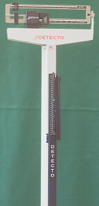
- With the help of your lab partner,
use the medical balance in the biology
lab to determine your height in centimeters (to the nearest 0.1 cm)
and your weight in kilograms (to the nearest 0.01 kg). You may wish
to remove your
shoes to obtain a more accurate height measurement. Make sure you obtain
readings with the correct number of decimal places, and make sure that you
record your data directly into your lab notebook.
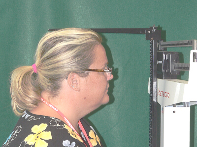
- To determine your height, raise the
height bar on the medical balance to approximately the height of your
head, then stand on the balance. Someone else should adjust the height
bar (up or down) until its arm sits flat on your head (make sure it is
pointing straight sideways and not slightly up or down).
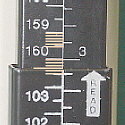
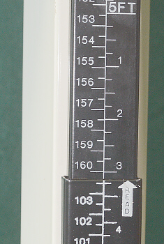
- Read your height
in the middle of the bar where the top piece slides into the bottom piece,
and make sure to use the metric scale. For example, the height shown in
these photos is 160.3 cm (not 5 ft 3⅛ in!). Also, remember to read
your height to the nearest 0.1 cm, and remember to record your data in your
lab notebook.
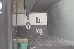
- When obtaining your weight, it is
important to notice that the beams on the medical balance have two
scales (metric and English) and two sets of notches intermixed. Begin
with the weighs on both beams set at 0.
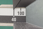
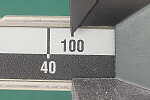
- First, adjust the weight on the lower
beam. You need to make sure that the weight is in a notch for one of the
metric system numbers, not one of the notches for an English system number
(notice the difference, here between the 40-kg and 100-lb notches). Adjust
the weight so that it is in the last metric notch thats too light.
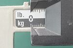
- Then, carefully slide the weight
on the top beam over to adjust the balance such that the needle swings the
same amount up and down. Do not wait for the needle to stop swinging because
friction may cause it to stop somewhere else.
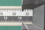
- Also, remember to read your weight
to the nearest 0.01 kg. This balance is at 14.15 kg, so added to the 40 kg
from the bottom beam, that persons total weight would be 54.15 kg.
- Remember to write all your numbers
in your lab notebook.
- Go to the
(biometrics Web page
and enter the requested data, including your name or initials, sex, age (to
the nearest 0.5 yr), height in centimeters (to the nearest 0.1 cm), and
weight in kilograms (to the nearest 0.01 kg) on that
page. Note: that page contains JavaScript code that is checking to see if
the right number of decimal places were entered, so if a message box pops
up, READ IT and do what it is asking you to do. When everyone has entered
his/her data, use the link at the bottom of that page to view and print a
copy of the class results so that you may subsequently analyze the
data.
How to Analyze Your Data
- After obtaining a copy of the
class data,
perform a statistical analysis on those data. Calculate the mean,
median, maximum, minimum, range, and standard deviation for age, height, and
weight for the last 10 males on the list and the last 10 females. Compare
the statistics for the males and females to determine whether there are any
sex-based differences in age, height, or weight. Calculate
the mean, median, maximum, minimum, range, and standard deviation for height
and weight for the last 10 people who are age 25 and under, and the last 10
people who are over 25. compare the statistics for the under-25 and over-25
groups to determine whether there are any age-based differences in height
or weight. Also, for the over-25 and under-25 groups, count the
number of males and females in each of those groups, and calculate what
percentages of each of those groups are male and female.
Make sure to enter all your work directly
into your lab notebook.
- For the groups to which you belong
(i.e. a 23-year-old male would do this for a) the males group and b)
the under-25 group), make histograms of the data as follows.
- First, make a list of ages,
by year (for example: 16.0 - 16.9, 17.0 - 17.9, etc.), from the
minimum to the maximum of those data. Secondly, make a list of
height by 5 cm categories (for example: 135.0 - 139.9, 140.0 - 144.9,
etc.) from the minimum to the maximum of those data. Thirdly, make a
list of weight by 10 kg categories (for example: 40.00 - 49.99, 50.00
- 59.99, etc.) from the minimum to the maximum of those data.
- For the last 100 people on
the whole class list who are the same sex as you, count/tally and
record the number of people in each age, height, and
weight category. (Thus, our example 23-year-old male would count the
number of males who fit into each of the 19, 20, etc. age categories,
the number of males who fit into each of the 150.0 - 154.9 cm,
etc. height categories, and the number of males who fit into
each of the 50.00 - 59.99, etc. kg weight categories.)
- For the last 100 people on
the whole class list who are the same over/under-25 age group as you,
count/tally and record the number of people in each height, weight,
and sex category. (Thus, our example 23-year-old male would count the
the number of under-25 people who fit into each of the height
and weight categories, as well as counting how many of the
under-25 people are male and how many are female.)
- Set up a histogram (graph)
for each comparison (i.e. our example 23-year-old male would
make histograms for ages of males, weight of males, height of males,
weight of under-25s, height of under-25s, and sex of under-25s). Each
block on the X-axis should represent one category (for example, on
the height histogram, one of the units on the X-axis would represent
the 150.0 - 154.9 cm group, the next would represent the 155.0 -
159.9 cm group, etc.). The Y-axis represents the number of people in
each category (for example, if 12 people were in the 60.00 - 69.99 kg
category, that bar would be 12 blocks tall). For each category listed
on the X-axis, draw a bar the appropriate height to represent the
number of people in that category. Refer to the graphing protocol
for information on proper graphing technique, and make sure to
properly title your graph and label the axes.
- For each graph except the
one for sex distribution, calulate the average (if you know how to
use your calculator or spreadsheet software to also calculate standard
deviation, you are encouraged to also do that).
On the X-axis, indicate where the mean would be located.
If you also calculated the standard deviation, indicate the position
of the mean + one standard deviation unit and the position of the
mean one standard deviation unit (for example, if
X = 5.00 and s = 0.20,
those two points would be at 5.20 and 4.80, respectively), as well as
the mean ± two standard deviation units (which would be 5.40 and 4.60
for this example).
- You should end up with
histograms for age distribution, height distribution, and weight
distribution for your sex and for height distribution, weight
distribution and sex for your over/under-25 age group (a total of 6
graphs).
- Compare your histograms with those
created by classmates of the opposite sex and/or in the opposite large age
group. How are they similar? Different? Are the means in the same places?
How similar or dissimilar are the standard deviations? Do any of the
histograms form a bell curve?
- Based on your statistical analysis of
the data, do there appear to any statistically-significant differences
in either age, height, or weight when comparing males vs. females or
differences in height or weight when comparing the over-25 and under-25 age
groups? For example,
if you have a group of data with a mean of 25 and a standard deviation of 3,
and another group of data with a mean of 22 with a standard deviation of 4,
those groups of data would not be different from each other. While
there is a fancy statistical calculation called a t-test that could be
done to determine whether these groups are different or not, for our
purposes, since 25 3 = 22 (higher average its standard deviation), and
22 + 4 = 26 (lower average + its standard deviation), and those numbers are
overlapping (22 = 22 and 26 > 25), it can be concluded that there is not
a statistically-significant difference between these numbers. If you were
doing an experiment and obtained these data for your control and experimental
groups, you would conclude that there is no difference between the groups,
the factor being tested in/on the experimental group had no effect as
compared to the control group. Thus, when stating your conclusions, it
is important to cite the actual numbers upon which those conclusions
are based.
- Before looking at the data, which
would you have expected to be more different between the under/over 25
groups: weight or height? Why? Do your data support or refute
this hypothesis?
- Complete the statistics practice
problems in the lab protocol. Show all your work in your lab notebook.
Other Things to Include in Your Notebook
Make sure you have all of the following in your lab notebook:
- all handout pages (in notebook or separate protocol book)
- all notes you take during the introductory mini-lecture
- all notes and data you gather as you perform the experiment
- your personal age-height-weight data
- print-out of class data (available online)
- all requested calculations based on class data
- all requested graphs based on class data
- answers to all discussion questions, a summary/conclusion in your
own words, and any suggestions you may have
- evidence that you have at least tried to work the practice
problems
- drawing of the medical balance used to obtain your height and
weight, including detail of exactly what the markings on the beams
actually look like
- any returned, graded pop quiz
Copyright © 2010 by J. Stein Carter. All rights reserved.
Based on printed protocol Copyright © 2000 J. L. Stein Carter.
This page has been accessed  times since 23 Jun 2011.