Climate
Climate Types
The following system of symbols (called the Trewartha
Modification of the Koppen Classification System) is one that is used to
classify various types of climates:
| A Tropical forest climates with no cool season; fairly constant warm temperature |
| Af: | constantly moist; rainfall all through the year |
| Aw: | distinct dry season in winter (Savanna). |
| Am: | monsoon rain; short, dry season, but with sufficient total rainfall to support rain forest |
| B Dry climates (precipitation variable and effectiveness dependent upon the rate of evaporation, which in turn, varies directly with temperature) |
| Bs: | semi-arid climates (Steppe) |
| Bw: | desert and arid climates (Wuste) |
| | h: | (heiss) tropical or low-latitude hot (heiss = German for hot) |
| | k: | (kalt) cold or middle-latitude (kalt = German for cold) |
| C Mesothermal (warm temperature) forest climates with cooler but mild winters (coldest month above 32° F [0° C]; warmest month above 50° F [10° C] (meso = middle; thermo = heat) |
| Cf: | no distinct dry season |
| Cw: | dry season in winter |
| Cs: | dry season in summer (Mediterranean type medi = middle; terra = earth, land) |
| | a: | hot summer (warmest month over 71.6° F [22° C]) |
| | b: | cool summer (warmest month under 71.6° F [22° C]) |
| | c: | cool, short summer; less that 4 months over 50° F [10° C] |
| D Microthermal (cold, snowy) forest climates with severe winters (coldest month below 32° F; warmest month above 50° F [10° C]) |
| Df: | no dry season |
| Dw: | dry winters |
| | a: | hot summer (warmest month over 71.6° F [22° C]) |
| | b: | cool summer (warmest month under 71.6° F [22° C]) |
| | c: | cool, short summer; less that 4 months over 50° F [10° C] |
| E Polar climates with no warm season (warmest month below 50° F [10° C]) |
| Et: | tundra climate (warmest month below 50° F [10° C], but above 32° F [0° C]) |
| Ef: | perpetual frost (all months below 32° F [0° C]); such climates persist only over the permanent ice caps |
Problem:
Consider the weather data for the cities listed in Table 1.
Classify the climatic types of these twelve cities using the Koppen symbols
(letters).
Hythergraphs
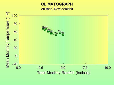
Figure 1. Climatograph for Aukland, N. Z.
Simple graphs can be constructed for an analysis of climate
and weather data. The method was originated in 1910 and first applied to a
practical problem in 1916. In constructing the graph, two related variables
are plotted on the graph paper. The vertical scale represents temperature
and the horizontal scale represents moisture (humidity or rainfall). The
monthly mean values are plotted as a series of points, one for each month
and the respective points are joined by a line in order of the months. The
polygon thus obtained is termed a
hythergraph
if temperature and rainfall are used, or a climatograph if temperature
and relative humidity are correlated. Climograph is a corruption of
the latter term, and has been used to mean both climatograph and hythergraph.
The time unit used may be any period (hour, week, day) but is usually month
or week.
For example, for Aukland, the climatograph would look like Figure 1.
Problem:
Plot hythergraphs for Barrow, Boston, Cuyaba, Delhi, and
Phoenix. Hythergraphs for Boston, Barrow, Cuyaba, and Delhi could probably
be put on the same graph with different symbols, while at least Delhi and
Phoenix will have to go on separate graphs because of overlapping data points.
Perhaps Barrow, Boston, and Delhi could go on one graph and Cuyaba and
Phoenix on another. Suggested scales are 20 to 100° F for temperature and
0 to 10 inches for precipitation. As time and interest allow, hythergraphs
for the other cities could also be constructed.
Hythergraphs, Continued
Hythergraphs also furnish a convenient means of comparing one
season with another. They are convenient and useful for giving a comparison
of the climate in a series of localities or to determine the probability
limits for the distribution of a particular species of organism. For,
example, a composite climatograph can be constructed for a locality or year
in which there were large numbers of a given species of insect and compared
to a climatograph for another locality or year in which no or few of that
species occurred. The index thus obtained is valuable in an analysis of the
influence of climatic variations upon the population size of that
species.
The data in Table 2 give mean temperature and monthly total
precipitation for two different years in an area of southern Illinois. The
first year was particularly favorable for a species of moth called the
codling moth (a fruit pest) and there were large numbers of these moths in
that year. The second year, there were few moths and they were not a
problem.
Table 2. Monthly Temperature and
Total Precipitation
for Two Years in a Southern Illinois Codling Moth
Area
| |
Moths Abundant |
Moths Scarce |
| Month |
(no.) |
Temp. (° F) |
Ppt. (inches) |
Temp. (° F) |
Ppt. (inches) |
| Jan |
1 |
35.5 |
0.8 |
36.0 |
1.7 |
| Feb |
2 |
26.0 |
2.7 |
28.0 |
1.7 |
| Mar |
3 |
40.0 |
1.8 |
42.0 |
4.9 |
| Apr |
4 |
53.0 |
3.1 |
53.5 |
5.3 |
| May 1st half |
5A |
59.0 |
2.6 |
N/A |
N/A |
| May 2nd half |
5B |
68.0 |
1.6 |
63.5 |
5.1 |
| Jun |
6 |
77.5 |
1.4 |
73.5 |
3.6 |
| Jul |
7 |
81.5 |
2.3 |
78.0 |
3.6 |
| Aug |
8 |
74.5 |
3.3 |
74.0 |
5.7 |
| Sep |
9 |
68.0 |
3.7 |
68.0 |
1.2 |
| Oct |
10 |
57.5 |
5.3 |
57.0 |
1.7 |
| Nov |
11 |
46.5 |
4.2 |
43.0 |
1.8 |
| Dec |
12 |
35.5 |
0.8 |
36.0 |
1.7 |
Problem:
Copyright © 1998 by J. Stein Carter. All rights reserved.
This page has been accessed  times since 26 Jun 2001.