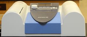
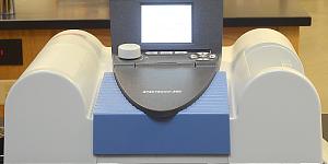
 Here is what the Spectronic 200 looks like (or should look like) when
it has just been obtained from where they are stored or when it is ready to
be stored. All the doors on the body are closed and the screen
is down.
Here is what the Spectronic 200 looks like (or should look like) when
it has just been obtained from where they are stored or when it is ready to
be stored. All the doors on the body are closed and the screen
is down.
Here is what the Spectronic 200 looks like (or should look like) when
it has just been obtained from where they are stored or when it is ready to
be stored. All the doors on the body are closed and the screen
is down.
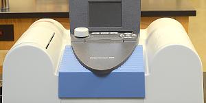 Here, the LCD screen has been tilted up so that it can easily be viewed.
The screen should be returned to its flat position prior to storage.
Here, the LCD screen has been tilted up so that it can easily be viewed.
The screen should be returned to its flat position prior to storage.
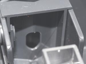
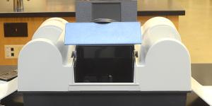 In this photo, the lid of the sample chamber has been raised to show
the location of the sample chamber, within. Also, if you look carefully, you
should be able to see that the doors to the cuvette-storage compartments
on the right and left sides have been opened.
In this photo, the lid of the sample chamber has been raised to show
the location of the sample chamber, within. Also, if you look carefully, you
should be able to see that the doors to the cuvette-storage compartments
on the right and left sides have been opened.
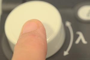
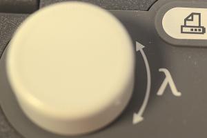 Across the top of the machine, in front of the screen, is a row of control
knobs and buttons. The left-most one of these is the wavelength knob
(or dial). Note that the symbol used to represent wavelength is the Greek
letter λ (lambda). Thus, in this Web page, the wavelength knob
will also be referred to as the λ knob. You may turn the
wavelength dial to adjust the wavelength by 10-nm intervals until youre
close to where you need to be.
Across the top of the machine, in front of the screen, is a row of control
knobs and buttons. The left-most one of these is the wavelength knob
(or dial). Note that the symbol used to represent wavelength is the Greek
letter λ (lambda). Thus, in this Web page, the wavelength knob
will also be referred to as the λ knob. You may turn the
wavelength dial to adjust the wavelength by 10-nm intervals until youre
close to where you need to be.
 Push down on the wavelength dial while turning it to fine-adjust the
wavelength by 1-nm intervals.
Push down on the wavelength dial while turning it to fine-adjust the
wavelength by 1-nm intervals.
Also notice in the above photo
that the button just to the
right of the wavelength knob is the Print Button. As of the writing
of this Web page, we did not, yet, have a printer for our Spec 200s, but we
are in the process of obtaining one. When that and/or the computer-interface
software are installed, you will be able to print a copy of your results.
 To the right of the print button is the Blank, or Auto-Zero Button
(here, also referred to as
0.00
to help you remember which button is being discussed). Since solvents such
as water and ethanol, as well as the plastic of which the cuvettes are made,
absorb some light, pushing the
0.00
button will zero the machine so it ignores any light absorbed by the
solvent and cuvette, and displays just the amount of light that is
absorbed by the specific substance being tested.
To the right of the print button is the Blank, or Auto-Zero Button
(here, also referred to as
0.00
to help you remember which button is being discussed). Since solvents such
as water and ethanol, as well as the plastic of which the cuvettes are made,
absorb some light, pushing the
0.00
button will zero the machine so it ignores any light absorbed by the
solvent and cuvette, and displays just the amount of light that is
absorbed by the specific substance being tested.
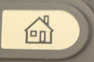 To the right of the blank/zero button is the Home Button (here, also
referred to as
⌂).
Pushing this button will send the Spec 200 back to its home menu display.
To the right of the blank/zero button is the Home Button (here, also
referred to as
⌂).
Pushing this button will send the Spec 200 back to its home menu display.
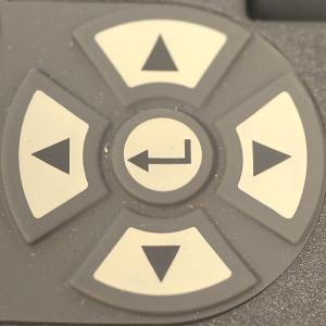 On the right-hand side of the top of the machine is a group of navigational
buttons. The four Arrow Buttons (▲=up, ►=right,
▼=down, and ◄=left) are used to navigate to various menu options
displayed on the screen.
The cEnter ↵ is the Enter Button, used to choose/execute
various options, just like on a computer.
On the right-hand side of the top of the machine is a group of navigational
buttons. The four Arrow Buttons (▲=up, ►=right,
▼=down, and ◄=left) are used to navigate to various menu options
displayed on the screen.
The cEnter ↵ is the Enter Button, used to choose/execute
various options, just like on a computer.
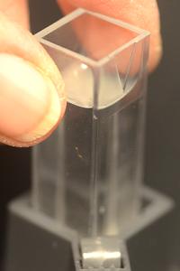
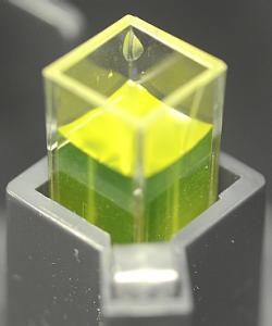
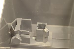 Heres a close-up of the Cuvette Holder within the sample chamber.
The Spec 200s Cuvettes are square plastic tubes that fit into
the holder. Note in the photo of the detector, below, the top edge of a
cuvette in place.
Heres a close-up of the Cuvette Holder within the sample chamber.
The Spec 200s Cuvettes are square plastic tubes that fit into
the holder. Note in the photo of the detector, below, the top edge of a
cuvette in place.
 The Light Source or Lamp is to the right, and shines its light
through the specimen in the cuvette.
The Light Source or Lamp is to the right, and shines its light
through the specimen in the cuvette.
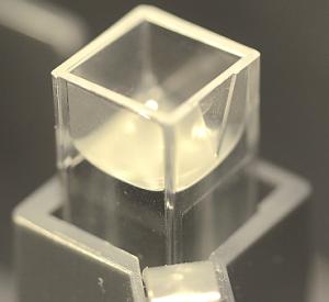
 To the left of the cuvette holder, there is a Detector which, as its
name suggests, detects the amount of light that is still left after passing
through the sample. The Spec 200s onboard computer then compares that with
the amount of light put out by the lamp to determine how much light was
absorbed by the specimen. Note that, because the machines calculations are
based on a comparison of the amount of light put out and the amount of light
left, its necessary to keep stray light out by keeping the lid of the
sample chamber shut.
To the left of the cuvette holder, there is a Detector which, as its
name suggests, detects the amount of light that is still left after passing
through the sample. The Spec 200s onboard computer then compares that with
the amount of light put out by the lamp to determine how much light was
absorbed by the specimen. Note that, because the machines calculations are
based on a comparison of the amount of light put out and the amount of light
left, its necessary to keep stray light out by keeping the lid of the
sample chamber shut.
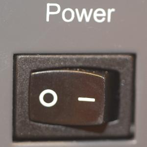 The Power Switch is located on the back of the Spec 200. After the
machine has been plugged in, the power may be switched on. A couple-minute
wait will be needed for the Spec 200s onboard computer to boot up.
Also, a USB Connector and a Printer Port are located on the
back if/when needed (but the Spec 200 can only talk to one certain kind
of small printer).
The Power Switch is located on the back of the Spec 200. After the
machine has been plugged in, the power may be switched on. A couple-minute
wait will be needed for the Spec 200s onboard computer to boot up.
Also, a USB Connector and a Printer Port are located on the
back if/when needed (but the Spec 200 can only talk to one certain kind
of small printer).
 When the Spectronic 200 is turned on, it will take a couple minutes for its
onboard computer to boot up.
When the Spectronic 200 is turned on, it will take a couple minutes for its
onboard computer to boot up.
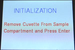 After the machines initial splash screen, it will display this initialization
screen which asks you to check to make sure someone else didnt leave a
cuvette in the sample compartment. Do check to make sure theres not one
in there, then make sure the lid is shut the machine needs that to correctly
calibrate itself on bootup. Once youre sure there in not a cuvette in the
chamber and that the door is shut, press the Enter (↵) button.
After the machines initial splash screen, it will display this initialization
screen which asks you to check to make sure someone else didnt leave a
cuvette in the sample compartment. Do check to make sure theres not one
in there, then make sure the lid is shut the machine needs that to correctly
calibrate itself on bootup. Once youre sure there in not a cuvette in the
chamber and that the door is shut, press the Enter (↵) button.
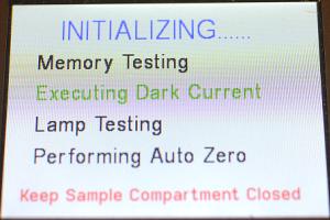 As the machine goes through its bootup sequence, it will display this
initialization screen to show what it is doing.
As the machine goes through its bootup sequence, it will display this
initialization screen to show what it is doing.
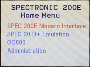 When it is done with its bootup, it will display its Home Screen. For
this course, we will use the Spec 200E Modern Interface Since that is
highlighted by default, just press Enter (↵) to go there.
After that, there will be several choices you will need to make, depending
on how the machine will be used.
When it is done with its bootup, it will display its Home Screen. For
this course, we will use the Spec 200E Modern Interface Since that is
highlighted by default, just press Enter (↵) to go there.
After that, there will be several choices you will need to make, depending
on how the machine will be used.
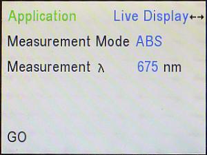 Heres what the Modern Interface Screen looks like. From this, you
will need to choose the option that is appropriate for the data to be
gathered. Note that the default Application is Live Display.
Heres what the Modern Interface Screen looks like. From this, you
will need to choose the option that is appropriate for the data to be
gathered. Note that the default Application is Live Display.
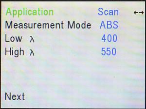
 For the Beers Law lab, there is one optional step that may
be done first, if desired. (If you are not doing this optional step,
skip
down to the instructions for setting the Application mode to Quant.)
Your protocol says to use a wavelength of 450 nm
for riboflavin, but do you wonder where that number came from? It really
wasnt just pulled out of thin air. If youd like to find that number for
yourself, use the right (►) and/or left (◄) arrows to
change from Live Display to Scan. The rest of what is displayed on
the screen changes accordingly. If Measurement Mode does not say ABS
(which stands for Absorbance), use the down (▼) arrow to go down to
the Measurement Mode line, and the right (►) and/or left (◄)
arrows to adjust it to ABS (for absorbance) it should not say, %T.
For the Beers Law lab, there is one optional step that may
be done first, if desired. (If you are not doing this optional step,
skip
down to the instructions for setting the Application mode to Quant.)
Your protocol says to use a wavelength of 450 nm
for riboflavin, but do you wonder where that number came from? It really
wasnt just pulled out of thin air. If youd like to find that number for
yourself, use the right (►) and/or left (◄) arrows to
change from Live Display to Scan. The rest of what is displayed on
the screen changes accordingly. If Measurement Mode does not say ABS
(which stands for Absorbance), use the down (▼) arrow to go down to
the Measurement Mode line, and the right (►) and/or left (◄)
arrows to adjust it to ABS (for absorbance) it should not say, %T.
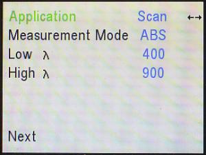
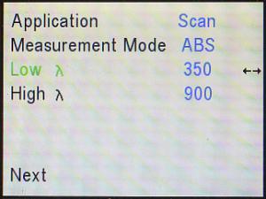
Then, use the down (▼) arrow to cursor down to Low λ
(remember λ stands for wavelength).
The default setting for the lowest wavelength it will use is 400 nm. Use the
wavelength (λ) knob and/or the right (►) and left
(◄) arrows to adjust that to 350 nm.
 Before |
 After |
|---|
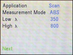
Similarly, use the down (▼) arrow to cursor down to High λ.
The default setting for the highest wavelength it will use is 900 nm. Use
the wavelength (λ) knob and/or right (►) and left
(◄) arrows to adjust that to 800 nm.
 Before |
 After |
|---|
 Then use the down (▼) arrow to cursor down to Next, and Enter
(↵) to go to the next screen.
Then use the down (▼) arrow to cursor down to Next, and Enter
(↵) to go to the next screen.
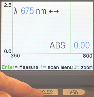
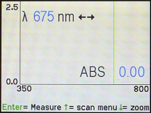 The next screen that will come up is an empty spectrum that looks like this.
 The next step is to blank the machine. Find a pair of plastic cuvettes
in one of the side compartments and because our samples are dissolved in
water, put water in one of them. Only
touch/hold the cuvettes by their top edges fingerprints on the area
through which the light travels will mess up the readings. If needed,
cuvettes may gently be polished with a piece of lens paper. Notice
that the top of one side of each cuvette has an arrow
(▽) on it. Always insert the cuvette with the arrow to the
right (toward the light source).
The next step is to blank the machine. Find a pair of plastic cuvettes
in one of the side compartments and because our samples are dissolved in
water, put water in one of them. Only
touch/hold the cuvettes by their top edges fingerprints on the area
through which the light travels will mess up the readings. If needed,
cuvettes may gently be polished with a piece of lens paper. Notice
that the top of one side of each cuvette has an arrow
(▽) on it. Always insert the cuvette with the arrow to the
right (toward the light source).
 Make sure the cuvette is all the way down and the arrow is on the right side
(toward the light source).
Make sure the cuvette is all the way down and the arrow is on the right side
(toward the light source).
 Then press the zero or blank
( 0.00 )
button so the machine can auto-zero itself (also referred to as blanking it).
Then press the zero or blank
( 0.00 )
button so the machine can auto-zero itself (also referred to as blanking it).
 While the machine is performing its auto-zero, it will display an hourglass
and a please wait message.
While the machine is performing its auto-zero, it will display an hourglass
and a please wait message.
 |
 |
 |
|---|
When the machine is done
with it calibration, remove the cuvette of water, and as was done with the
water, place some of the riboflavin solution from the tube of your most
concentrated solution into a second
cuvette. Insert the cuvette into the cuvette holder, making sure the arrow
points to the right. Make sure the cuvette is all the way in and close the
lid. Then, press Enter (↵) to determine at what wavelength
riboflavin absorbs the most light.
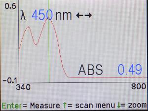 The Spec 200 will measure and display the spectrum for riboflavin, which
should look similar to this. However, the
green line that is the Cursor may be over at the far left (or anywhere
else on your graph). Use the wavelength (λ) dial and/or
right (►) and left (◄) arrows to move the green cursor line until
it exactly matches with the top of the highest peak. Notice that, as the
cursor is moved, the machine will display what wavelength (λ) it is
on and the corresponding absorbance (ABS) for that wavelength. Notice
that the highest light absorbance is at (or very close to) 450 nm. That is
why the instructions in the protocol say to use 450 nm (hopefully, your
data correspond to this). You may photograph this spectrum to include in
your lab notebook (or if the new printer is working, print out a copy).
The Spec 200 will measure and display the spectrum for riboflavin, which
should look similar to this. However, the
green line that is the Cursor may be over at the far left (or anywhere
else on your graph). Use the wavelength (λ) dial and/or
right (►) and left (◄) arrows to move the green cursor line until
it exactly matches with the top of the highest peak. Notice that, as the
cursor is moved, the machine will display what wavelength (λ) it is
on and the corresponding absorbance (ABS) for that wavelength. Notice
that the highest light absorbance is at (or very close to) 450 nm. That is
why the instructions in the protocol say to use 450 nm (hopefully, your
data correspond to this). You may photograph this spectrum to include in
your lab notebook (or if the new printer is working, print out a copy).
 Use the up (▲) arrow to return to the Application screen.
Change the application from Scan to Quant. A number of options will
appear on the screen. No. of STDs means number of standards, and the
machine will only allow a maximum of 4. If it does not already say 4,
cursor down to that line and change it to 4. If the Measurement Mode does
not already say ABS, cursor down to that line and change it to ABS. If the
Measurement λ does not already say, 450 (if you followed the
previous instructions, it should remember whatever wavelength the green
cursor line was on when you left Scan) cursor down to that line, and change
it to 450 nm. The way were expressing concentration (milliliters of
riboflavin solution added) doesnt really correspond to the machines choices
of Unit, so if its saying something like C, you can just leave it there.
Dont worry about the line that says, USB Memory. When everything is
properly set, cursor down to Go, and press Enter (↵) to
continue to the next screen.
Use the up (▲) arrow to return to the Application screen.
Change the application from Scan to Quant. A number of options will
appear on the screen. No. of STDs means number of standards, and the
machine will only allow a maximum of 4. If it does not already say 4,
cursor down to that line and change it to 4. If the Measurement Mode does
not already say ABS, cursor down to that line and change it to ABS. If the
Measurement λ does not already say, 450 (if you followed the
previous instructions, it should remember whatever wavelength the green
cursor line was on when you left Scan) cursor down to that line, and change
it to 450 nm. The way were expressing concentration (milliliters of
riboflavin solution added) doesnt really correspond to the machines choices
of Unit, so if its saying something like C, you can just leave it there.
Dont worry about the line that says, USB Memory. When everything is
properly set, cursor down to Go, and press Enter (↵) to
continue to the next screen.
Next, the Spec 200 will ask you to insert a cuvette of blank
solution (in this case, water) into the cuvette holder and press the Auto
Zero button. Refer to the instructions, above, for proper insertion of
the cuvette. When the machine is done with that, it will display a screen
with spaces for the four standards to be tested. Use your plain water
(again) as your first standard (0 riboflavin should absorb 0 light), as
well as your 0.2 mL, 0.7 mL and 1.0 mL tubes for the other three standards.
For each standard, cursor up or down until youre on that line.
Use the right (►) and left (◄) arrows to set the concentration
for that sample (to 0.0 or 0.2 or 0.7 or 1.0 as appropriate). Then, press
Enter (↵) to analyze that sample. The Spec 200 will put the
absorbance reading into the last column. As you do each of your samples,
write down the absorbance reading obtained for each specimen into your lab
notebook. Then, cursor down to the next sample and repeat the process.
In between samples, you may remove the cuvette, pour the sample that in
the cuvette back into its test tube, then pour the next sample into the
cuvette, insert it back into the sample chamber, close the lid, and take a
reading. Do not rinse the cuvette with water in between samples as any
remaining water droplets in the cuvette will dilute the sample thats in
the cuvette, thus causing the absorbance reading to be wrong.
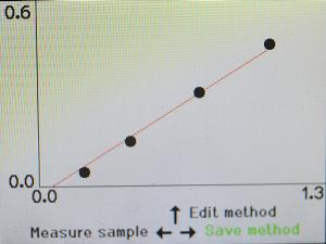 When you have measured all four of those samples, the machine will give you
the option to press Enter (↵) to display the Beers Law curve.
Note that it will calculate a best-fit straight line from your data, but
the object of the game, here, is to be so good at pipetting that all of
your data points fall exactly on the line, not a bit to one side or the
other. Notice that the points on the graph in this photo do not all fall
right on the line: some are above and some are below. How close to a
straight line did you come? You may photograph (or print if available) your
graph to include in your lab notebook.
When you have measured all four of those samples, the machine will give you
the option to press Enter (↵) to display the Beers Law curve.
Note that it will calculate a best-fit straight line from your data, but
the object of the game, here, is to be so good at pipetting that all of
your data points fall exactly on the line, not a bit to one side or the
other. Notice that the points on the graph in this photo do not all fall
right on the line: some are above and some are below. How close to a
straight line did you come? You may photograph (or print if available) your
graph to include in your lab notebook.
To analyze your 0.1 and 0.4 mL samples, one at a time, place
each of those into a cuvette and into the Spec 200. Note at the bottom of
the display screen, it says Measure Sample ←. Press Enter
(↵) to analyze that sample. The machine will display its
absorbance (please write that down in your lab notebook), and a concentration
reading (as though that sample was an unknown) based on the best-fit line
that it calculated (so unless you had phenomenal pipetting technique, that
will not exactly match with 0.1 or 0.4 mL but, hopefully, will come close).
Determine the absorbance of those two samples by that means.
Since there are usually about six samples to be tested in this
lab exercise, one way of doing this that has worked well in the past is for
the class to divide up into six (or however many pigments there are) groups,
and each group adopt a pigment and a spectrophotometer. That way, the
spectrum from each pigment can be displayed on its own spectrophotometer, and
all students can, then, go from machine to machine examining (and photographing)
the spectra. (However, if/when we do get a printer and/or computer interface
that is/are only hooked up to one Spec 200, that will change what works best.)
Due to the way our old Spec 20s worked, the lab protocol for
the Photosynthesis Lab includes instructions to obtain absorbance readings
for all pigments at 350 nm, then to change to 375 nm, re-blank, and test
all pigments there, then 400 nm, etc., but with these new Spec 200s, all of
that is no longer needed, and by following the instructions, below, it is
actually quicker and easier to obtain the data needed to construct a
spectrum for each pigment, one by one.
For the spectra of photosynthetic pigments, start by setting the Spec 200 to
scan mode. That is the same mode described above, to find the absorption
peak for riboflavin, so many of the directions here are identical to the
directions given there.
As above, use the right (►) and/or left (◄) arrows to
change from Live Display to Scan. The rest of what is displayed on
the screen changes accordingly. If Measurement Mode does not say ABS
(which stands for Absorbance), use the down (▼) arrow to go down to
the Measurement Mode line, and the right (►) and/or left (◄)
arrows to adjust it to ABS (it should not say, %T).
Then, use the down (▼) arrow to cursor down to Low λ.
The default setting for the lowest wavelength it will use is 400 nm. Use the
wavelength (λ) knob and/or the right (►) and left
(◄) arrows to adjust that to 350 nm.
Before |
After |
|---|
Similarly, use the down (▼) arrow to cursor down to High λ.
The default setting for the highest wavelength it will use is 900 nm. Use
the wavelength (λ) knob and/or right (►) and left
(◄) arrows to adjust that to 800 nm.
Before |
After |
|---|
Then use the down (▼) arrow to cursor down to Next, and Enter
(↵) to go to the next screen.
Again, the next screen that will come up looks like this.
The next step is to blank the machine. Find a pair of plastic cuvettes
in one of the side compartments and put ETHANOL (do you know why you
should use that and not water?) in one of them. Only
touch/hold the cuvettes by their top edges fingerprints on the area
through which the light travels will mess up the readings. If needed,
cuvettes may gently be polished with a piece of lens paper. Notice
that the top of one side of each cuvette has an arrow
(▽) on it. Always insert the cuvette with the arrow to the right.
Make sure the cuvette is all the way down and the arrow is on the right side.
Then press the zero
( 0.00 )
button so the machine can auto-zero itself.
While the machine is performing its auto-zero, it will display an hourglass
and a please wait message.
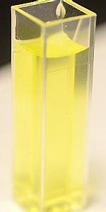
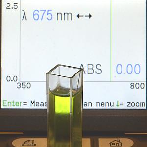 Then its ready to analyze your samples, so put one in. For example, here
is a sample of parsley extract, ready to be put into the sample chamber.
Then its ready to analyze your samples, so put one in. For example, here
is a sample of parsley extract, ready to be put into the sample chamber.
 As was done with the ethanol, pour some of the solution of the pigment you
wish to study from the test tube into a second cuvette. Insert the cuvette
into the cuvette holder, making sure the arrow points to the right. Make
sure the cuvette is all the way in and close the lid. Then, press Enter
(↵) to display the absorption spectrum for that pigment.
The machine will display the message, Scanning... with an hourglass.
As was done with the ethanol, pour some of the solution of the pigment you
wish to study from the test tube into a second cuvette. Insert the cuvette
into the cuvette holder, making sure the arrow points to the right. Make
sure the cuvette is all the way in and close the lid. Then, press Enter
(↵) to display the absorption spectrum for that pigment.
The machine will display the message, Scanning... with an hourglass.
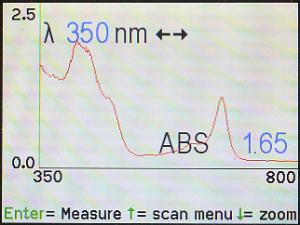 Here is the resulting spectrum for the parsley extract used above. Note that
the cursor is on 350 nm.
Here is the resulting spectrum for the parsley extract used above. Note that
the cursor is on 350 nm.
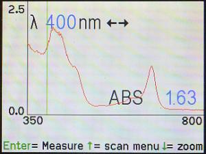 The wavelength (λ) knob and/or the right (►) and left
(◄) arrows may be used to move to another part of the spectrum. Here,
the cursor is on 400 nm, and the machine says that, at that wavelength, the
absorbance is 1.63.
The wavelength (λ) knob and/or the right (►) and left
(◄) arrows may be used to move to another part of the spectrum. Here,
the cursor is on 400 nm, and the machine says that, at that wavelength, the
absorbance is 1.63.
Your protocol book instructs you to graph the data from the pigment(s) you
tested. To do that, you will first need to make a chart of the numbers you
will need to construct the graph. Start with a list, going down the page, of
all the wavelengths to be used (350, 370, 400, 425 nm, etc.). Then another
column will be needed (down the page) for each pigment tested. Use the
wavelength (λ) knob and/or the left (◄) and right
(►) arrows to move the green cursor line over by 25-nm
increments (350, 375, 400, 425 nm, etc.), up to 800 nm. At each of those
wavelengths, students should copy the reported absorbance into their
lab notebooks. The protocol book explains how to use those absorbance
numbers to construct a graph. Your graph should look similar to the spectrum
that is displayed on the Spec 200s screen, with the big difference that, on
your graph, you will know what the actual numbers are.
 Here to the left, the cursor has been moved to what appears to be a peak at 415 nm, and
the machine says that, at that wavelength, the absorbance is 2.01. This
actually is a bit tricky because this is a parsley leaf extract that contains
a mixture of pigments: chlorophylls A and B, carotenes, xanthophylls, etc.,
Here to the left, the cursor has been moved to what appears to be a peak at 415 nm, and
the machine says that, at that wavelength, the absorbance is 2.01. This
actually is a bit tricky because this is a parsley leaf extract that contains
a mixture of pigments: chlorophylls A and B, carotenes, xanthophylls, etc.,
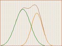 so what is seen here is an additive spectrum of all those put together
(similar to the diagram on the right).
Thus, while 415 nm appears to be a peak, it may, in fact, be due to
the additive effect of several pigments whose peaks are actually at slightly
different wavelengths: while their peaks are at other places, the sides
of those peaks may add up to give an apparent peak here.
so what is seen here is an additive spectrum of all those put together
(similar to the diagram on the right).
Thus, while 415 nm appears to be a peak, it may, in fact, be due to
the additive effect of several pigments whose peaks are actually at slightly
different wavelengths: while their peaks are at other places, the sides
of those peaks may add up to give an apparent peak here.
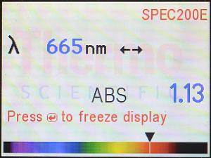
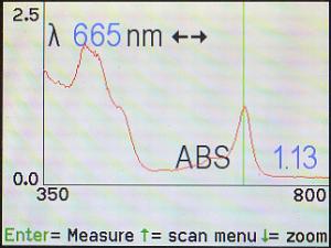 Here, the cursor has been moved to the other peak at 665 nm. The
machine is saying that, at that wavelength, the absorption is 1.13.
Use the wavelength (λ) knob and/or the left (◄)
and right (►) arrows to move the green cursor line to the
highest point on each of the absorbance peaks (hint: watch for the highest
ABS as the green cursor line is moved back and forth).
Make note of each of those wavelengths and absorbance readings in your lab
notebook. Those numbers may then be compared with published max/min numbers.
Here, the cursor has been moved to the other peak at 665 nm. The
machine is saying that, at that wavelength, the absorption is 1.13.
Use the wavelength (λ) knob and/or the left (◄)
and right (►) arrows to move the green cursor line to the
highest point on each of the absorbance peaks (hint: watch for the highest
ABS as the green cursor line is moved back and forth).
Make note of each of those wavelengths and absorbance readings in your lab
notebook. Those numbers may then be compared with published max/min numbers.
 This method can also be used to determine areas of minimal light absorbance.
For example, here, the cursor has been moved to 525 nm where there appears
to be a minimum. The machine is reporting that the absorbance is only 0.02
at that point. However, its difficult to tell whether the cursor is at the
absolute lowest point. One way to determine that is by slowly moving the
cursor back and forth while watching for the lowest absorbance (ABS) reading.
This method can also be used to determine areas of minimal light absorbance.
For example, here, the cursor has been moved to 525 nm where there appears
to be a minimum. The machine is reporting that the absorbance is only 0.02
at that point. However, its difficult to tell whether the cursor is at the
absolute lowest point. One way to determine that is by slowly moving the
cursor back and forth while watching for the lowest absorbance (ABS) reading.
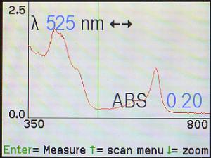
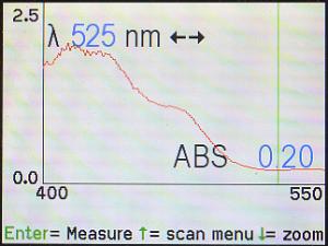 The Spec 200 has another feature that can help in this situation. Notice
in the photo, above, at the bottom of the screen, it says to push the
down (▼) arrow to zoom to a higher magnification. Here, with the
cursor on 525 nm, the down (▼) arrow was pressed, with the result that
the machine is displaying only the section from 400 to 550 nm. The
disadvantage to using zoom is that there is no un-zoom feature, and the
only way to get out of zoom view is to press the up (▲) arrow to go
all the way back to the Scan menu, then ask the machine to regenerate the
spectrum.
The Spec 200 has another feature that can help in this situation. Notice
in the photo, above, at the bottom of the screen, it says to push the
down (▼) arrow to zoom to a higher magnification. Here, with the
cursor on 525 nm, the down (▼) arrow was pressed, with the result that
the machine is displaying only the section from 400 to 550 nm. The
disadvantage to using zoom is that there is no un-zoom feature, and the
only way to get out of zoom view is to press the up (▲) arrow to go
all the way back to the Scan menu, then ask the machine to regenerate the
spectrum.
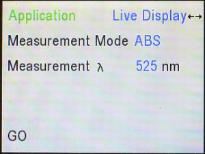 The Spec 200 also gives us a means of seeing what color of light corresponds
to a given wavelength. Here, with the cursor left on 525 nm (or whatever
wavelength you wish to examine), the
up (▲) arrow was pressed to go back to the Scan Menu, and back from
that to the Application Menu. There, Scan may be changed to Live Display,
as shown here.
The Spec 200 also gives us a means of seeing what color of light corresponds
to a given wavelength. Here, with the cursor left on 525 nm (or whatever
wavelength you wish to examine), the
up (▲) arrow was pressed to go back to the Scan Menu, and back from
that to the Application Menu. There, Scan may be changed to Live Display,
as shown here.
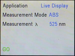 Then, use the down (▼) arrow key to cursor to where it says, GO and
press the Enter (↵) key to do it.
Then, use the down (▼) arrow key to cursor to where it says, GO and
press the Enter (↵) key to do it.
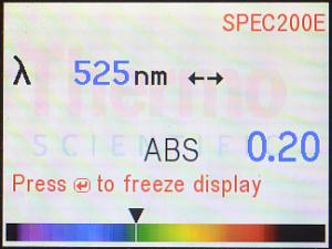 Here is the resulting display for 525 nm. Its still saying that the absorbance
at 525 nm is 0.20. Notice the rainbow (spectrum) across the bottom of the
screen, and especially notice where the arrow (▼) is pointing. The
color of the spectrum at that point indicates (as best as possible on an LCD
screen) the color of light which corresponds to that wavelength: 525 nm is
green light, which plants do not absorb (which is why they look green
to us).
Here is the resulting display for 525 nm. Its still saying that the absorbance
at 525 nm is 0.20. Notice the rainbow (spectrum) across the bottom of the
screen, and especially notice where the arrow (▼) is pointing. The
color of the spectrum at that point indicates (as best as possible on an LCD
screen) the color of light which corresponds to that wavelength: 525 nm is
green light, which plants do not absorb (which is why they look green
to us).
 You can also check the color that corresponds to other areas of the spectrum,
especially including the peaks. If you have written down the wavelength(s)
of the peak(s), you can use the wavelength (λ) dial and/or
the right (►) and left (◄) arrow keys to go to that wavelength.
If you do not know or remember the wavelength whose color you wish to
determine, you will need to go back to the Application Menu, back into Scan,
re-scan the pigment (re-do the spectrum), move the cursor over the desired
wavelength, and then go back to Live Display.
You can also check the color that corresponds to other areas of the spectrum,
especially including the peaks. If you have written down the wavelength(s)
of the peak(s), you can use the wavelength (λ) dial and/or
the right (►) and left (◄) arrow keys to go to that wavelength.
If you do not know or remember the wavelength whose color you wish to
determine, you will need to go back to the Application Menu, back into Scan,
re-scan the pigment (re-do the spectrum), move the cursor over the desired
wavelength, and then go back to Live Display.
 428 nm |
 665 nm |
|---|
Here are the displays (for the same parsley solution) for
428 nm (which your lecture textbook says is the absorption max for
Chlorophyll A) and 665 nm (the location of the smaller peak. According to
this display, 428 nm corresponds to blue-violet, and 665 nm corresponds to
red (your lecture textbook probably mentioned that, too). This way, youve
seen it for yourself, rather than just reading about it.
Again, because we currently do not have printers available, it is, thus, not
possible (yet) to print out a copy of the spectrum graph as displayed by the
machine. Thus, students who have a camera or cell phone with built-in camera
should be encouraged to photograph the screen showing the spectrum for the
pigment they tested (hint: if six groups of students each test one of the
pigments on a different spectrophotometer, it would be very easy for everyone
to go around to all the spectrophotometers and take a picture of the spectrum
for each of the six pigments, so everyone could have the whole set), and
include a print-out of it/all of them in their lab notebook.
However, that is not a substitute in place of learning the proper method for
construction of a graph, so a properly-done, hand-drawn graph should be
constructed.
If a second (or more) pigment is to be tested, just remove the
first cuvette of pigment and insert the new cuvette/pigment to be tested,
then press the Enter (↵) button to generate a spectrum for the
new pigment. As above, these absorbance readings can be added as another
column on the chart/table students have created in their lab notebooks
and subsequently used to create a graph for that pigment.
Depending on how your chromatography turned out, your class
should have test tubes of the redissolved, individual pigments: carotene,
xanthophyll 1, xanthophyll 2, Chlorophyll A, Chlorophyll B, and the
center spot that did not move. Obtain an absorption spectrum for each of
those pigments and any others which your class may be testing (and photograph
for inclusion in your lab notebook or print out if printer is available).
In your lab notebook, record the wavelength (nm) of the absorption maxima
(tips of peaks) and minima (bottoms of valleys) for each of the pigments.
Be very careful in your observations for example,
Chlorophyll A will probably show a peak around 425 to 428 nm, and that is,
actually, significantly different from carotenes peak at around 450 nm.
Refer to the lists at the end Beers Law and Photosynthetic Pigments lab Web pages for lists of items that should be included for each of those labs.